Elinear: linear algebra basics in Clojure
Table of Contents
Preface
This text is primarily my personal notes on linear algebra as I go through Matrix Analysis & Applied Linear Algebra. At the same time this document is a literate program that can be executed in Emacs so the text will be slowly building up a linear algebra library of sorts. This will often not match the order things are presented in the book. There is no emphasis on performance - just on clarity, extensability and correctness when possible. This is purely (self)educational with my primary motivation being to help me better understand what I learn (through having to explain it) and to sanity check with actual programs. Things that are adequately explained in the book will not be repeated here.
This is my first program in Elisp, so if you see any issues, please leave a note in the issues tab of the repository. There you can also find the original org-mode file and the generated elisp files - both of which have additional unit-tests ommited from this webpage.
This is very much a work in progress and will change often…
Systems of linear equations
The book's opening problem from ancient China of calculating the price of bushels of crop serves as a good example of a linear problem. I've simplified the problem a bit for clarity - but I will expand on it and refer back to it extensively:
A farming problem
You have a 3 fruit farms in a region of ancient China. In a given year:
Given 1:
Farm 1 produces 3 tons of apples 2 ton of oranges and 1 ton of lemons
Farm 2 produces 2 tons of apples 3 tons of oranges and 1 ton of lemons
Farm 3 produces 1 ton of apples 2 tons of oranges and 3 tons of lemons
Given 2:
Farm 1 sold its fruit for 39 yuan
Farm 2 sold its fruit for 34 yuan
Farm 3 sold its fruit for 26 yuan
What is the price of the a ton of apples/oranges/lemons?
This is a familiar problem that can be restated as a system of linear equations
\begin{equation} \begin{split} 3x+2y+z = 39\\ 2x+3y+z = 34\\ x+ 2y + 3z = 26 \end{split} \end{equation}
Where x, y and z represent apples oranges and lemons respectively
We know how to solve this system by manipulating the equations, solving for a variable and then back-substituting the results.
It's not accident I split up the problem into two sets of Givens. It's important to note that the problem actually has two distinct and independent parts. There is the farm/crop linear system (Given 1), and then there is the constraint of the profits of each farm (Given 2)
We are looking for the input fruit-prices that will yield the given profits for each farm
Matices as representations of linear systems
The linear system can be represented with a matrix
\begin{bmatrix} 3 & 2 & 1\\ 2 & 3 & 1\\ 1 & 2 & 3\\ \end{bmatrix}or flipped::
\begin{bmatrix} 3 & 2 & 1\\ 2 & 3 & 2\\ 1 & 1 & 3\\ \end{bmatrix}We prefer the first representation, but both ways work as long as you remember what each row and column represents
The Matrix in the computer
Once we've chosen a layout the easiest way to store the matrix in the computer is to remember 3 values: number-of-rows number-of-columns data
The data value will be a long list of size num-row * num-col that contains all the values of the matrix; row after row. So given a list data and a pair of sizes we simply build the matrix into a list of these three values:
(defun matrix-from-data-list (number-of-rows number-of-columns data-list)
  "Builds a matrix from a data list"
  (list
   number-of-rows
   number-of-columns
   data-list))
Some helpers
With a couple of helper function we can get back these 3 fields. This will improve the readability of the code as we go along
(defun matrix-rows (matrix)
  "Get the number of rows"
  (nth 0 matrix))
(defun matrix-columns (matrix)
  "Get the number of columns"
  (nth 1 matrix))
(defun matrix-data (matrix)
  "Get the data list from the matrix"
  (nth 2 matrix))
(defun matrix-get-value (matrix row column)
  "Get the scalar value at position ROW COLUMN (ZERO indexed) from MATRIX"
  (nth
   (+
    column
    (*
     row
     (matrix-columns matrix)))
    (matrix-data matrix)))
nthgets the nth element of the list
For debugging and looking at results we also need to be able to print out the matrix for inspection
(defun matrix-data-get-first-n-values (data n)
  "Given a list of values, get the first n in a string"
  (if (zerop n)
      "" ;base case
    (concat
     (number-to-string (car data))
     " "
     (matrix-data-get-first-n-values (cdr data) (1- n))))) ;iterative step

(defun matrix-data-print (number-of-rows number-of-columns data)
  "Print out the data list gives the dimension of the original matrix"
  (if (zerop number-of-rows)
      "" ;base case
    (concat
     (matrix-data-get-first-n-values data number-of-columns)
     "\n"
     (matrix-data-print ;iterative step
      (1- number-of-rows)
      number-of-columns
      (nthcdr number-of-columns data )))))

(defun matrix-print (matrix)
  "Print out the matrix"
  (concat "\n" (matrix-data-print
                (matrix-rows matrix)
                (matrix-columns matrix)
                (matrix-data matrix))))
; ex:  (message (matrix-print (matrix-from-data-list 2 2 '(1 2 3 4))))
zeroptests if the value is zero
()with a quote is the empty-list
consattaches the first argument to the second argument (which is normally a list)
cdrreturns the list without the first element
Transposition: Getting the other equivalent matrix
Since we have two equivalent matrices that represent our linear system we need a mechanism to go from one to the other. This method is the matrix transpose which flips the matrix along the diagonal. The text goes into depth on the properties of the matrix transpose, but in short, as long as you take the transpose of both sides of your equations equivalances will be preserved.
(defun matrix-transpose (matrix)
  "Get the transpose of a matrix"
  (if (equal (matrix-columns matrix) 1)
    (matrix-from-data-list
     1
     (matrix-rows matrix)
     (matrix-data matrix))
    (matrix-append
     (matrix-from-data-list
      1
      (matrix-rows matrix)
      (matrix-data (matrix-get-column matrix 0)))
     (matrix-transpose
      (matrix-submatrix
       matrix
       0
       1
       (matrix-rows matrix)
       (matrix-columns matrix))))))
Representing the whole system of equations
Now that we can represent the fruit/profits system we want a mechanism to represent the whole system of equations so that given a constraint, we can solve for a solution.
Matrix Multiplication
This is done notationally with matrix multiplication. The notation allows us to keep the two Givens separated and allows us to visually chain linear systems together. As a shorthand, we write the product of two matrices A and B as AB = C, with the order of A and B being important. For every value (at a given row and column position) in the resulting matrix C we take the equivalent row in A and multiply it by its equivalent column in B. From this we can conclude that C will have as many rows as A and as many column as B
Multiplying a row times a column is called an inner product
Inner Product
The inner-product is defined as the sum of the product of every pair of equivalent elements in the two vectors. The sum will naturally return one scalar value. This operation only makes sense if both the row and column have the same number of values.
(defun matrix-inner-product-data (row-data column-data)
  "Multiply a row times a column and returns a scalar. If they're empty you will get zero"
  (reduce
   '+
   (for-each-pair
    row-data
    column-data
   '*)))

(defun matrix-inner-product (row column)
  "Multiply a row times a column and returns a scalar. If they're empty you will get zero"
  (matrix-inner-product-data
   (matrix-data row)
   (matrix-data column)))
reduceworks down the list elements-by-element applying the operator on each cumulative result
Submatrices
To get rows and columns (and other submatrices) we need a few more helper functions
(defun matrix-extract-subrow (matrix row start-column end-column)
  "Get part of a row of a matrix and generate a row matrix from it. START-COLUMN is inclusive,  END-COLUMN is exclusive"
  (let
      ((number-of-columns-on-input (matrix-columns matrix))
       (number-of-columns-on-output (-
                                     end-column
                                     start-column)))
    (matrix-from-data-list
     1
     number-of-columns-on-output
     (subseq
      (matrix-data matrix)
      (+ (* row number-of-columns-on-input) start-column)
      (+ (* row number-of-columns-on-input) end-column)))))

(defun matrix-append (matrix1 matrix2)
  "Append one matrix (set of linear equations) to another"
  (if (null matrix2)
      matrix1
    (matrix-from-data-list
     (+
      (matrix-rows matrix2)
      (matrix-rows matrix1))
     (matrix-columns matrix1)
     (append
      (matrix-data matrix1)
      (matrix-data matrix2)))))

(defun matrix-submatrix (matrix start-row start-column end-row end-column)
  "Get a submatrix. start-row/column are inclusive. end-row/column are exclusive"
  (if (equal start-row end-row)
      '()
    (matrix-append
     (matrix-extract-subrow matrix start-row start-column end-column)
     (matrix-submatrix
      matrix
      (1+ start-row)
      start-column
      end-row
      end-column))))

(defun matrix-get-row (matrix row)
  "Get a row from a matrix. Index starts are ZERO"
  (matrix-extract-subrow
   matrix
   row
   0
   (matrix-columns matrix)))

(defun matrix-get-column (matrix column)
  "Get a column from a matrix. Index starts are ZERO"
  (matrix-submatrix
   matrix
   0
   column
   (nth 0 matrix)
   (1+ column)))
Matrix Product
Now we have all the tools we need to write down the algorithm for calculating the matrix product. First we write a function to calculate the product for one value at a given position
(defun matrix-product-one-value (matrix1 matrix2 row column)
  "Calculate one value in the resulting matrix of the product of two matrices"
  (matrix-inner-product
   (matrix-get-row matrix1 row )
   (matrix-get-column matrix2 column)))
And then we recursively apply it to construct the resulting matrix
(defun matrix-product (matrix1 matrix2)
  "Multiply two matrices"

  (defun matrix-product-rec (matrix1 matrix2 row column)
    "A recursive helper function that builds the matrix multiplication's data vector"
    (if (equal (matrix-rows matrix1) row)
        '()
      (if (equal (matrix-columns matrix2) column)
          (matrix-product-rec
           matrix1
           matrix2
           (1+ row)
           0)
        (cons
         (matrix-product-one-value
          matrix1
          matrix2
          row column)
         (matrix-product-rec
          matrix1
          matrix2
          row
          (1+ column))))))

  (matrix-from-data-list
   (matrix-rows matrix1)
   (matrix-columns matrix2)
   (matrix-product-rec
    matrix1
    matrix2
    0
    0)))
Matrix Conformability
You will notice that the algorithm won't make sense if the number of columns of A doesn't match the number of rows of B. When the values match the matrices are called conformable. When they don't match you will see that inner product isn't defined and therefore neither is the product.
(defun matrix-conformable? (matrix1 matrix2)
  "Check that two matrices can be multiplied"
  (equal
   (matrix-columns matrix1)
   (matrix-rows matrix2)))
Addendum: Scalar Product
An additional form of matrix multiplication is between a matrix and a scalar. Here we simply multiply each element of the matrix times the scalar to construct the resulting matrix. The order of multiplication is not important -> αA=Aα
(defun matrix-scalar-product (matrix scalar)
  "Multiple the matrix by a scalar. ie. multiply each value by the scalar"
  (matrix-from-data-list
   (matrix-rows matrix)
   (matrix-columns matrix)
   (mapcar
   (lambda (x)
     (* scalar x))
   (matrix-data matrix))))
A system of equations as matrix product
Now that we have all our tools we can write down a matrix product that will mimic our system of equation.
\begin{equation} \begin{bmatrix} 3 & 2 & 1\\ 2 & 3 & 1\\ 1 & 2 & 3\\ \end{bmatrix} \begin{bmatrix} x\\ y\\ z\\ \end{bmatrix} = \begin{bmatrix} 39\\ 34\\ 26\\ \end{bmatrix} \end{equation}Going through our algorithm manually we see that the resulting matrix is:
\begin{equation} \begin{bmatrix} 3x + 2y + z\\ 2x + 3y + z\\ x + 2y + 3z\\ \end{bmatrix} = \begin{bmatrix} 39\\ 34\\ 26\\ \end{bmatrix} \end{equation}The mirror universe
Now I said that flipped matrix was also a valid representation. We can confirm this by taking the transpose of both sides
\begin{equation} \begin{bmatrix} x & y & z\\ \end{bmatrix} \begin{bmatrix} 3 & 2 & 1\\ 2 & 3 & 2\\ 1 & 1 & 3\\ \end{bmatrix} = \begin{bmatrix} 39 & 34 & 26\\ \end{bmatrix} \end{equation}It yields another matrix product that mimics the equations, however you'll see in the textbook that we always prefer the first notation.
Chaining problems through matrix composition
The real power of matrix multiplication is in its ability to chain systems together through linear composition
If we are given a new problem that take the output of our first system and produces a new output - composition gives us a mechanism to combine the systems into one.
Taxing our farmers
Say the imperial palace has a system for collecting taxes
Given:
The farms have to pay a percentage of their income to different regional governements. The breakdown is as follows:
The town taxes Farm 1 at 5%, Farm 2 at 3%, Farm 3 at 7%
The province taxes all Farm 1 at 2% Farm 2 at 4%, Farm 3 at 2%
The palace taxes all farms at 7%
Now, given the income of each farm i we can build a new matrix B and calculate the tax revenue of each government - t.
From the previous problem we know that the income of each farm was already a system of equation with the price of fruit as input f
So we just plug one into the other and get
and compose a new equation that given the price of fruit gives us the regional tax revenue. By carrying out the product we can generate one linear system
Where if BA=C the final composed system is:
\begin{equation} Cf=t \end{equation}Note that the rows of BA are the combination of the rows of A and the columns of BA are the combination of the columns of B - at the same time! (see page 98)
EXAMPLE: Geometrical transformations
A very simple example are the linear systems that takes coordinates x y and do transformations on them
Rotation
\begin{equation} \begin{bmatrix} \cos \theta & -\sin \theta \\ \sin \theta & \cos \theta \\ \end{bmatrix} \begin{bmatrix} x \\ y \\ \end{bmatrix} = \begin{bmatrix} x_{rotated}\\ y_{rotated}\\ \end{bmatrix} \end{equation}(defun matrix-rotate-2D (radians) "Generate a matrix that will rotates a [x y] column vector by RADIANS" (matrix-from-data-list 2 2 (list (cos radians) (- (sin radians)) (sin radians) (cos radians))))
Reflection about X-Axis
\begin{equation} \begin{bmatrix} 1 & 0 \\ 0 & -1\\ \end{bmatrix} \begin{bmatrix} x \\ y \\ \end{bmatrix} = \begin{bmatrix} x_{reflected}\\ y_{reflected}\\ \end{bmatrix} \end{equation}(defun matrix-reflect-around-x-2D () "Generate a matrix that will reflect a [x y] column vector around the x axis" (matrix-from-data-list 2 2 '(1 0 0 -1)))
Projection on line
\begin{equation} \begin{bmatrix} 1/2 & 1/2 \\ 1/2 & 1/2\\ \end{bmatrix} \begin{bmatrix} x \\ y \\ \end{bmatrix} = \begin{bmatrix} x_{projected}\\ y_{projected}\\ \end{bmatrix} \end{equation}(defun matrix-project-on-x=y-diagonal-2D () "Generate a matrix that projects a point ([x y] column vector) onto a line (defined w/ a unit-vector)" (matrix-from-data-list 2 2 '(0.5 0.5 0.5 0.5)))
So given a point [x y] (represented by the column vector v) we can use these 3 transformation matrices to move it around our 2D space. We simple write a chain of transformations T and multiply them times the given vector T1T2T3v=vnew. These transformation matrices can then be multiplied together into one that will carry out the transformation in one matrix product. T1T2T3=Ttotal => Ttotalv=vnew
Equivalent matrices
Now thanks to matrix multiplication we can represent linear systems and we can chain them together. The next step is extending multiplication to represent general manipulations of matrices.
Identity Matrix
For any matrix A, the identity matrix I is such that A*I = A = I*A. Given the dimensions, I has to be a square matrix. It will have 1's on the diagonal (ie. where row==column) and zeroes everywhere else. We build it recursively:
(defun matrix-identity (rank)
  "Build an identity matrix of the given size/rank"

  (defun matrix-build-identity-rec (rank row column)
    "Helper function that build the data vector of the identity matrix"
    (if (equal column rank) ; time to build next row
        (if (equal row (1- rank))
            '() ; we're done
          (matrix-build-identity-rec
           rank
           (1+ row)
           0))
      (if (equal row column)
          (cons
           1.0
           (matrix-build-identity-rec
            rank
            row
            (1+ column)))
        (cons
         0.0
         (matrix-build-identity-rec
          rank
          row
          (1+ column))))))

  (matrix-from-data-list rank rank (matrix-build-identity-rec rank 0 0 )))
Unit Column/Rows
Each column of the identity matrix is a unit column (denoted as ej). It contains a 1 in a given postion (here: j) and 0s everwhere else. Its transpose is naturally called the unit row
Aej = the j column of A
eiTA = the i row of A
eiTAej = gets the [ i, j ] element in A
(defun matrix-unit-rowcol-data (index size)
"Create a data-list for a matrix row/column. INDEX (starts at ZERO) matches the row or column where you want a 1. SIZE is the overall size of the vector"
(if (zerop size)
    '()
  (if (zerop index)
      (cons
       1.0
       (matrix-unit-rowcol-data
        (1- index)
        (1- size)))
    (cons
     0.0
     (matrix-unit-rowcol-data
      (1- index)
      (1- size))))))
(defun matrix-unit-column (row size)
  "Build a unit column. ROW is where you want the 1 to be placed (ZERO indexed). SIZE is the overall length"
      (matrix-from-data-list
       size
       1
       (matrix-unit-rowcol-data
        row
        size)))
(defun matrix-unit-row (column size)
  "Build a unit column. COLUMN is where you want the 1 to be placed (ZERO indexed). SIZE is the overall length"
      (matrix-from-data-list
       1
       size
       (matrix-unit-rowcol-data
        column
        size)))
Here I'm just trying out a new notation. With
letrecwe can hide the recursive helper function inside the function that uses it.
Addition
As a tool in building new matrices, we need a way to easily add two matrices, ie. add their values one to one. Matrices that are added need to have the same size.
(defun matrix-equal-size-p (matrix1 matrix2)
  "Check if 2 matrices are the same size"
  (and
   (equal
    (matrix-rows matrix1)
    (matrix-rows matrix2))
   (equal
    (matrix-columns matrix1)
    (matrix-columns matrix2))))
(defun for-each-pair (list1 list2 operator)
  "Go through 2 lists applying an operator on each pair of elements"
  (if (null list1)
      '()
    (cons
     (funcall operator (car list1) (car list2))
     (for-each-pair (cdr list1) (cdr list2) operator))))

(defun matrix-add (matrix1 matrix2)
  "Add to matrices together"
  (if (matrix-equal-size-p matrix1 matrix2)
      (matrix-from-data-list
       (matrix-rows matrix1)
       (matrix-columns matrix1)
       (for-each-pair
        (matrix-data matrix1)
        (matrix-data matrix2)
        '+))))

(defun matrix-subtract (matrix1 matrix2)
  "Subtract MATRIX2 from MATRIX1"
  (if (matrix-equal-size-p matrix1 matrix2)
      (matrix-from-data-list
       (matrix-rows matrix1)
       (matrix-columns matrix1)
       (for-each-pair
        (matrix-data matrix1)
        (matrix-data matrix2)
        '-))))
funcallapplied the first arugment (a function) with the remaining items in the list as arguments
Elementary Matrices
The manipulation of the rows and columns can be broken down into 3 types of elementary matrices that when multiplied with our linear systems will generate equivalent matrices (E).
(from page 134)
When applied from the left EA=B it performs a row operation and makes a row equivalent matrix.
When applied from the right AE=B it performs a column operation and makes a column equivalent matrix.
Row/column operations are ofcourse reversible and therefore E is invertible and a E-1 always exists.
So now, waving our hands a little, given a non-singular matrix we can restate Gauss-Jordan elimination as "a bunch of row operations that turn our matrix into the identity matrix". Ie: Ek..E2E1A=I
And thanks to each operations' invertibility we can flip it to be A=E1-1E2-1..Ek-1
So Gauss-Jordan elimination for non-singular matrices has given us our first decomposition of sorts! We now know that every non-singular matrix can be written as a chain of row (or column) operations.
Row/Column operations come in 3 flavors
Type I - Row/Column Interchange
Interchaning rows (or columns) i and j
(defun matrix-elementary-interchange (rowcol1 rowcol2 rank)
  "Make an elementary row/column interchange matrix for ROWCOL1 and ROWCOL2 (ZERO indexed)"
  (let ((u
         (matrix-subtract
          (matrix-unit-column rowcol1 rank)
          (matrix-unit-column rowcol2 rank))))
  (matrix-subtract
   (matrix-identity rank)
   (matrix-product
    u
    (matrix-transpose u)))))

(defun matrix-elementary-interchange-inverse (rowcol1 rowcol2 rank)
  "Make the inverse of the elementary row/column interchange matrix for ROWCOL1 and ROWCOL2 (ZERO indexed). This is identical to (matrix-elementary-interchange)"
  (matrix-elementary-interchange
   rowcol1
   rowcol2
   rank))
Type II - Row/Column Multiple
Multiplying row (or column) i by α
(defun matrix-elementary-multiply (rowcol scalar rank)
  "Make an elementary row/column multiple matrix for a given ROWCOL (ZERO indexed)"
  (let ((elementary-column
         (matrix-unit-column rowcol rank)))
  (matrix-subtract
   (matrix-identity rank)
   (matrix-product
    elementary-column
    (matrix-scalar-product
     (matrix-transpose elementary-column)
     (- 1 scalar))))))

(defun matrix-elementary-multiply-inverse (rowcol scalar rank)
  "Make the inverseof the elementary row/column multiple matrix for a given ROWCOL (ZERO indexed)"
  (matrix-elementary-multiply
   rowcol
   (/ 1 scalar)
   rank))
Type III - Row/Column Addition
Adding a multiple of a row (or column) i to row (or column) j
(defun matrix-elementary-addition (rowcol1 rowcol2 scalar rank)
  "Make an elementary row/column product addition matrix. Multiply ROWCOL1 (ZERO indexed) by SCALAR and add it to ROWCOL2 (ZERO indexed)"
  (matrix-add
   (matrix-identity rank)
   (matrix-scalar-product
    (matrix-product
     (matrix-unit-column rowcol2 rank)
     (matrix-transpose
      (matrix-unit-column rowcol1 rank)))
    scalar)))

(defun matrix-elementary-addition-inverse (rowcol1 rowcol2 scalar rank)
  "Make the inverse of the elementary row/column product addition matrix. Multiply ROWCOL1 (ZERO indexed) by SCALAR and add it to ROWCOL2 (ZERO indexed)"
  (matrix-elementary-addition
   rowcol1
   rowcol2
   (- scalar)
   rank))
The LU Decomposition
Gaussian elimination in matrix form
If linear equations at their simplest take inputs and produce some outputs, then Gaussian elimination is our method of reversing the process. It's a systematic way for taking a known linear system with a given output and solving for its input. Because we know that adding and scaling equations preserves equalities, Gaussian elimination is a scheme for combining and swapping equations so that they reduce to something simpler which can be solved directly. We do this by elimination factors in our equations such that the last one is of the form αx=b. Equalities being preserved, we can use this simple equation to solve for one of the unknown inputs. Each of the remaining equation includes just one additional unknow input so that through back-substitution we can then solve for all of them one by one.
So if Ax=b is our original system of equations in matrix form, then after Gaussian elimination we can write our simplified systm as Ux=bnew. Combining our equations has changed our output values, so the b has changes as well.
From the Example on page 141
So if we started with an A that looked like this
Gaussian elimination will give us a U that look like this:
\begin{bmatrix} 2 & 2 & 2\\ 0 & 3 & 3\\ 0 & 0 & 4\\ \end{bmatrix}Looking at the system of equations Ux=bnew and given a bnew we can see that the last row in U - [ 0 0 4 ] times the column [ x1 x2 x3 ]T gives us a direct solution for x3. Then using x3 and the previous row/equation we could solve for x2 and so on.
Combining and swapping rows is something we just learned how to do using elementary matrices- so by cleverly taking their product with our matrix A we will be able to generate the U matrix - in effect reenacting Gaussian elimination using matrix multiplication. If each row manipulation is some elementary matrix Rn we could write out the process of Gaussian elimination as a series of products RnR…R2R1A=U. Looking at Ax=b it's just the same - we simply multiply by both sides by the R matrices RnR…R2R1(Ax)=R1R2R…Rnb. As we were hoping for, the left side will be Ux and the right hand side is our bnew.
On a high level the reduction of the equations happens in two repeated steps on each column: First we adjust the pivot and then we eliminate all the factors below it. In the matrix representation this is equivalent to adjusting the diagonal element and then making all the values below it equal to zero. The combination of the two reduces the column and make our system simpler.
Note: Gaussian elimination will only produce a solution for nonsingular square matrices, so the process described only holds for this case
Elementary Lower Triangular Matrics
The example I used above was done without adjusting any pivots. We reducing the first column by simply eliminated the values below the 2 (in the upper left) and we could have done that by multiply our A by two Type III elementary matrices from the left like so:
The two Type III elementary matrices on the left are pretty simple and you can visually see what the -2 and -3 represent. They match the entry in A at the same index (row/column), but divided by the value of the pivot (ie: the factor that will eliminate the value). The result is that the first column has been reduced and we are closer to our upper triangular U
Constructing these simple Type III matrices is quick and inverting them is as easy as flipping the sign on the factor (ie. if you subtract some multiple of an equation from another, to reverse the operation you'd simply add the same multiple of the equation back)
(defun matrix-elementary-row-elimination (matrix row column)
  "Make a matrix that will eliminate an element at the specified ROW/COLUMN (ZERO indexed) using the diagonal element in the same column (typically the pivot)"
  (let
      ((pivot (matrix-get-value matrix column column))
       (element-to-eliminate (matrix-get-value matrix row column)))
    (matrix-elementary-addition
     column
     row
     (-
      (/
       element-to-eliminate
       pivot))
     (matrix-rows matrix))))
Looking again at the product of 2 Type III matrices with our A, and using what we know about composing linear systems, we already know that we can take the product of the first two matrices separately. Whatever matrix comes out we can then multiply times A to give us the same result.
The result is surprisingly simple and we can see that we didn't really need to carry out the whole matrix product b/c we've simply merged the factors into one matrix. So we can simply build these matrices that eliminate entire columns and skip making tons of Type III matrices entirely. The new combined matrices are called Elementary Lower-Triangular Matrix and are described on page 142.
(defun matrix-elementary-lower-triangular (matrix column-to-clear)
  "Make a matrix that will eliminate all rows in a column below the diagonal (pivot position)"

  (defun matrix-elementary-lower-triangular-rec (matrix column-to-clear row-to-build rank)
    "Recursive function to build the elementary lower triangular matrix"
    (cond
     ((equal
       rank
       row-to-build) ; Done building the matrix
      '())
     ((<=
       row-to-build
       column-to-clear) ; Building the simply "identity" portion above the pivot
      (matrix-append
       (matrix-unit-row row-to-build rank)
       (matrix-elementary-lower-triangular-rec
        matrix
        column-to-clear
        (1+ row-to-build)
        rank)))
     (t ; Build the elimination portion below the pivot
      (let
          ((pivot (matrix-get-value matrix column-to-clear column-to-clear))
           (element-to-eliminate (matrix-get-value matrix row-to-build column-to-clear)))
        (let
            ((cancellation-factor (-
                                   (/
                                    element-to-eliminate
                                    pivot))))
          (matrix-append
           (matrix-add
            (matrix-unit-row row-to-build rank)
            (matrix-scalar-product
             (matrix-unit-row column-to-clear rank)
             cancellation-factor))
           (matrix-elementary-lower-triangular-rec
            matrix
            column-to-clear
            (1+ row-to-build)
            rank)))))))

  (matrix-elementary-lower-triangular-rec
   matrix
   column-to-clear
   0
   (matrix-rows matrix)))
Building the L Matrix
So now our product of elementary matrices RnR…R2R1A=U shortens to something similar GrG…G2G1A=U, but where each Elementary Lower-Triangular Matrix G takes the place of several R matrices. The product GrG…G2G1 involved a lot of matrix products, but fortunately we have a shortcut. These G matrices have the property that their inverse is just a matter of flipping the sign of the factors' in their column. You can confirm this by inverting our definition G=RnR…R2R1 and remembering that the R's just involve a sign flip and R-1's are also Type III matrices.
(defun matrix-invert-elementary-lower-triangular (matrix-elementary-lower-triangular)
  "Inverts an L matrix by changing the sign on all the factors below the diagonal"
  (matrix-add
   (matrix-scalar-product
    matrix-elementary-lower-triangular
    -1)
   (matrix-scalar-product
    (matrix-identity
     (matrix-rows matrix-elementary-lower-triangular))
    2)))
TODO: Add a function to build the inverse directly
This allows us to take our equation G1G2G…GnA=U and trivially produce the interesting equality A=G-11G-12G-1…GnU without having to compute a single value; just flip the order of the product and flup the signs. Now the product G-11G-12G-1…Gn is special and page 143 describes how all the factors just move into one matrix without having to do any calculation. (Note: that the same doesn't hold for the non-inverted product of the G's!) The combined product produces the lower triangular matrix L and lets us write down A=LU - from which we get the name of the decomposition. (see page 143-144 eq 3.10.6 )
To finish our example we will first add another matrix to the left to eliminate the second column in A so that we have the equation G2G1A=U
\begin{equation} \begin{bmatrix} 1 & 0 & 0\\ 0 & 1 & 0\\ 0 & -4 & 1\\ \end{bmatrix} \begin{bmatrix} 1 & 0 & 0\\ -2 & 1 & 0\\ -3 & 0 & 1\\ \end{bmatrix} \begin{bmatrix} 2 & 2 & 2\\ 4 & 7 & 7\\ 6 & 18 & 22\\ \end{bmatrix} = \begin{bmatrix} 2 & 2 & 2\\ 0 & 3 & 3\\ 0 & 0 & 4\\ \end{bmatrix} \end{equation}Note that the factor of
\begin{bmatrix} 2 & 2 & 1\\ 0 & 3 & 3\\ 0 & 12 & 16\\ \end{bmatrix}-4was only deduced after doing the reduction of the first column which had given us:So you can't reduce the second column before you'd reduced the first!
Next we invert our two 2 G matrices and bring them to other side to get A=G1-1G2-1U (Notice how the order of the G's has changed b/c of the inversion)
\begin{equation} \begin{bmatrix} 2 & 2 & 2\\ 4 & 7 & 7\\ 6 & 18 & 22\\ \end{bmatrix} = \begin{bmatrix} 1 & 0 & 0\\ 0 & 1 & 0\\ 0 & 4 & 1\\ \end{bmatrix} \begin{bmatrix} 1 & 0 & 0\\ 2 & 1 & 0\\ 3 & 0 & 1\\ \end{bmatrix} \begin{bmatrix} 2 & 2 & 2\\ 0 & 3 & 3\\ 0 & 0 & 4\\ \end{bmatrix} \end{equation}Now multiplying the two inverted matrices is quick and easy b/c we just need to merge the factors into one matrix:
\begin{equation} \begin{bmatrix} 2 & 2 & 2\\ 4 & 7 & 7\\ 6 & 18 & 22\\ \end{bmatrix} = \begin{pmatrix} \begin{bmatrix} 1 & 0 & 0\\ 0 & 1 & 0\\ 0 & 4 & 1\\ \end{bmatrix} \begin{bmatrix} 1 & 0 & 0\\ 2 & 1 & 0\\ 3 & 0 & 1\\ \end{bmatrix} \end{pmatrix} \begin{bmatrix} 2 & 2 & 2\\ 0 & 3 & 3\\ 0 & 0 & 4\\ \end{bmatrix} \end{equation} \begin{equation} \begin{bmatrix} 2 & 2 & 2\\ 4 & 7 & 7\\ 6 & 18 & 22\\ \end{bmatrix} = \begin{bmatrix} 1 & 0 & 0\\ 2 & 1 & 0\\ 3 & 4 & 1\\ \end{bmatrix} \begin{bmatrix} 2 & 2 & 2\\ 0 & 3 & 3\\ 0 & 0 & 4\\ \end{bmatrix} \end{equation}And we are left with A=LU
When we do this is code we immediately invert the G's and build up their product. So as we eliminate A column after column and turn it into the upper triangular U we are in parallel accumulating the inverse of the elimination matrices into L. The function will return us two matrices, L and U
(defun matrix-LU-decomposition (matrix)
  "Perform Gaussian elimination on MATRIX and return the list (L U), representing the LU-decomposition. If a zero pivot is hit, we terminate and return a string indicating that"
  (let
      ((rank
        (matrix-rows matrix)))
    (defun matrix-LU-decomposition-rec (L-matrix
                                        reduced-matrix
                                        column-to-eliminate)
      (cond
       ((equal column-to-eliminate rank)
        (list L-matrix reduced-matrix))
       ((zerop
         (matrix-get-value
          reduced-matrix
          column-to-eliminate
          column-to-eliminate))
        "ERROR: LU decomposition terminated due to hitting a zero pivot. Consider using the PLU")
       (t
        (let ((column-elimination-matrix (matrix-elementary-lower-triangular
                                          reduced-matrix
                                          column-to-eliminate)))
          (matrix-LU-decomposition-rec
           (matrix-product
            L-matrix
            (matrix-invert-elementary-lower-triangular
             column-elimination-matrix))
           (matrix-product
            column-elimination-matrix
            reduced-matrix)
           (1+ column-to-eliminate))))))

    (matrix-LU-decomposition-rec
     (matrix-identity rank)
     matrix
     0)))
TODO: I'm updating L by doing a a product here (ie. Lnew = G-1Lold).. but the whole point is that L can be updated without a product. This could use a helper function that would build/update L's
Updating U could also be done without doing a whole matrix product and just looking at the lower submatrix
Partial Pivoting
Now while in previous section we managed to decompose A into two matrices L and U, you may have noticed there is an error condition our code. The issue is that we may find that after performing elimination on a column we are left with a zero in the next column's pivot position. This makes it impossible to eliminate the factors below it. The solution we have from Gaussian Elimination is to swap in a row from below so that the pivot is non-zero. We are going to take advantage of this and use the strategy called partial pivoting and will swap in to the pivot position whichever row has the maximal value for that column. It will ensure that our results have less error and like any row-swap can be done pretty easily with a Type I elementary matrix.
(defun matrix-partial-pivot (matrix pivot-column)
    "Returns a Type-I matrix that will swap in the row under the pivot that has maximal magnititude"
    (let ((column-below-pivot (matrix-submatrix
                               matrix
                               pivot-column
                               pivot-column
                               (matrix-rows matrix)
                               (1+ pivot-column))))
      (defun find-max-index (data-list max-val max-index current-index)
        (cond
         ((null data-list)
          max-index)
         ((>
           (abs(car data-list))
           max-val)
          (find-max-index
           (cdr data-list)
           (abs(car data-list))
           current-index
           (1+ current-index)))
         (t
          (find-max-index
           (cdr data-list)
           max-val
           max-index
           (1+ current-index)))))

     (matrix-elementary-interchange
      pivot-column
      (+
       pivot-column
       (find-max-index
        (matrix-data column-below-pivot)
        0
        0
        0))
      (matrix-rows matrix))))
So if Gn were the elementary lower-triangular matrices from the last section that performed our eliminations and Fn are the new Type I pivot adjustments then if we adjust our pivot before each elimination, our reduction needs to be rewritten as G1F1G2F2..GrFrA=U where each G F pair corresponds to a reduction of a column: (G1F1)col1(G2F2)col2..(GrFr)colrA=U.
(defun matrix-reduce-column (matrix column-to-reduce)
  "Adjusts the pivot using partial pivoting and eliminates the elements in one column. Returns a list of the elimination matrix, permutation matrix and the resulting matrix with reduced column (list of 3 matrices)"
  (let*
      ((pivot-adjusting-matrix
        (matrix-partial-pivot
         matrix
         column-to-reduce) )
       (matrix-with-partial-pivoting
        (matrix-product ; pivot!
         pivot-adjusting-matrix
         matrix))
       (column-elimination-matrix
        (matrix-elementary-lower-triangular
         matrix-with-partial-pivoting
         column-to-reduce))
       (matrix-with-reduced-column
        (matrix-product ; reduce
         column-elimination-matrix
         matrix-with-partial-pivoting)))
    (list column-elimination-matrix pivot-adjusting-matrix matrix-with-reduced-column)))
TODO: Return G-1 instead, because it's more directly what we need later
Turning back to our orginal Ax=b we can again generate the bnew: Ux=(G1F1)col1(G2F2)col2..(GrFr)colrb -> Ux=bnew. Then again using back substitution we can get a solution for x…. However this solution has some serious flaws. Looking at (G1F1)col1(G2F2)col2..(GrFr)colr we can no longer use the inversion trick to copy factors together. We seem to be foreced to carry out a whole lot of matrix products. Before we added the pivots in, we had manage to get a clean equation A=LU, and L was especially easy to make without carrying out a single matrix product - but now building that decomposition suddenly isn't as easy!
Extracting the pivots
On page 150 the book shows us how we can fix this situation by extracting the partial pivots out of column reductions so that instead of: G1F1G2F2..GrFrA=U we are left with something that looks more like G1G2..GrF1F2..FrA=U. With the G's together we can use our inversion trick to get our easily-computed L back. Then taking the product of the F's gives us a new permutation matrix P so that our final equation will look like PA=LU. Looking at the book's solution from a different perspective, the reason we've had the matrices interleaved is because that's how we build them (from right to left). We can't go into the middle of the matrix and adjust the pivot position till we'd carried out all the eliminations in the columns before it. The previous eliminations will mix up the rows and change all the values in that column so the maximal value won't be known ahead of time. So the GFGFGF sequence for building the reduction matrices (from right to left, column by column) needs to be observed. The trick is that once we've finished Gaussian elimination then we know the final order of the rows in U and what page 150 demonstrates is that if we know the row interchanges, we can actually carry them out first as long as we then fix-up any preceding eliminations matrices a bit. Specifically if you adjust some pivot k by swapping it with row k+i then any previous eliminations that involved the row k (and row k+i) now needs to be fixed to reflect that you'll be doing the row interchange ahead of time.
While the G1G2..GrF1F2..FrA=U representation is really handy, we would like to build matrices as-we-go and not have to build the interleaved mess and then have to spend time fixing it.
The strategy is that as we pivot-adjust and eliminate and pivot-adjust and eliminate column by column, slowly building up our U matrix, each time we pivot-adjust we build our permuation matrix P by accumulating the products of the F's and we fix-up the preceeding eliminations. The way it's described in the book, they seem to update all the G matrices that came before - however my shortcut is to skip all the G's and go straight to building the L matrix and to adjust the rows there. Just as before with the plain LU decompostion, every G we get during elimination is inverting it to G-1, and then added it to L so that Lnew = LoldG-1. The extra step is that now each time we adjust a pivot with a new F we update L such that Lnew=FLoldF.
To see why this is equivalent to updating all the G's and then inverting at the end, rememeber that F=F-1 b/c a row exchange is it's own inverse. So F2=I. So if we have are in the middle of Gaussian elimination and have G3G2G1A=U and we then do a pivot adjustment FG3G2G1A=U then we can insert a identity matrix FG3G2G1IA=U expand it to FF so that FG3G2G1FFA=U then bring everything to the other side FA=F-1G1-1G2-1G3-1F-1U recover our easy-to-compute L matrix FA=F-1LF-1U simplify our F-1's so that FA=FLFU and we have our new L in FA=LnewU ie. Lnew=FLoldF
(defun matrix-update-L-matrix (elementary-lower-triangular-matrix type-i-interchange-matrix)
  "Take an elementary lower triangular matrix and update it to match a row interchange between ROW1 and ROW2 (ZERO indexed)"
    (matrix-product
     type-i-interchange-matrix
     (matrix-product
      elementary-lower-triangular-matrix
      type-i-interchange-matrix)))
TODO: Update to not do two full matrix products. This can be do with some clever number swapping instead
So our method will still go reducing the matrix column by column and building up U, but in parallel we will be building L and P. So the result will be the three matrices (P L U).
(defun matrix-PLU-decomposition (matrix)
  "Perform Gaussian elimination with partial pivoting on MATRIX and return the list (P L U), representing the LU-decomposition "
  (let
      ((rank
        (matrix-rows matrix)))
    (defun matrix-PLU-decomposition-rec (P-matrix
                                        L-matrix
                                        reduced-matrix
                                        column-to-reduce)
      (cond
       ((equal
         column-to-reduce
         rank)
        (list P-matrix L-matrix  reduced-matrix))
       (t
        (let
            ((current-column-reduction-matrices
              (matrix-reduce-column
               reduced-matrix
               column-to-reduce)))
          (matrix-PLU-decomposition-rec
           (matrix-product                              ; update the permutation matrix
            (second current-column-reduction-matrices)
            P-matrix)
           (matrix-product
            (matrix-update-L-matrix       ; update elimination matrices due to partial pivot
             L-matrix
             (second current-column-reduction-matrices))
            (matrix-invert-elementary-lower-triangular (first current-column-reduction-matrices)))
           (third current-column-reduction-matrices)    ; the further reduced matrix
           (1+ column-to-reduce))))))

    (matrix-PLU-decomposition-rec
     (matrix-identity rank)
     (matrix-identity rank)
     matrix
     0)))
Using the LU
Notes on getting a good numerical solution:
Section 1.5 goes into a good amount of detail of why floating point arithmetic will introduce errors and how to mitigate the problem. Partial pivoting will provide a bit of help, however it's also suggested to use row-scaling and column-scaling.
Row-scaling will alter the magnitude of the output value of your linear system, while column scaling will alter the scale of your inputs. Don't hesitate to have the inputs and outputs use different units. page 28 suggests scaling the rows such that the maximum magnitude of each row is equal to 1 (ie. divide the row by the largest coefficient)
The topic of residuals, sensitivity and coditioning will be revisited later
Solving for x in Ax=b
Now that we can break a linear system A into two systems L and U we need to go back to where we started and solve for inputs given some outputs.We started with Ax=b and now we know we can do PA=LU. Combinding the two we can get PAx=Pb and then LUx=Pb. As mentioned before, bnew=Pb, so for simplicity LUx=bnew. The new b has the same output values, just reordered a bit due to pivot adjustments. Since the order of the original equations generally doesn't have a special significance this is just a minor change.
Next we define a new intermediary vector Ux=y so that we can write Ly=bnew. This value we can solve directly by forward substitution. The first row of the lower triangular matrix gives us a simple solvable equation of the form ax=b and every subsequent row adds an additional unknown that we can solve for directly.
(defun matrix-forward-substitution (lower-triangular-matrix output-vector)
  "Solve for an input-vector using forward substitution. ie. solve for x in Lx=b where b is OUTPUT-VECTOR and L is the LOWER-TRIANGULAR-MATRIX"
  (defun matrix-forward-substitution-rec (lower-triangular-matrix input-vector-data output-vector-data row)
    (cond
     ((null output-vector-data) ;; BASE CASE
      input-vector-data)
     (t                         ;; REST
      (matrix-forward-substitution-rec
       lower-triangular-matrix
       (append
        input-vector-data
        (list
         (/
          (-
           (car output-vector-data)
           ;; on the first iteration this is the product of null vectors.. which in our implementation returns zero
           (matrix-inner-product-data
            (matrix-data
             (matrix-extract-subrow
              lower-triangular-matrix
              row
              0
              row))
            input-vector-data))
          (matrix-get-value lower-triangular-matrix row row))))
       (cdr output-vector-data)
       (1+ row)))))

  (matrix-from-data-list
   (matrix-rows lower-triangular-matrix)
   1
   (matrix-forward-substitution-rec
    lower-triangular-matrix
    '()
    (matrix-data output-vector)
    0)))
Once we have y we can go to Ux=y and solve for x by back substitution
(defun matrix-back-substitution (upper-triangular-matrix output-vector)
  "Solve for an input-vector using forward substitution. ie. solve for x in Lx=b where b is OUTPUT-VECTOR and L is the LOWER-TRIANGULAR-MATRIX"
  (matrix-from-data-list
   (matrix-rows upper-triangular-matrix)
   1
   (reverse
    (matrix-data
     (matrix-forward-substitution
      (matrix-from-data-list
       (matrix-rows upper-triangular-matrix)
       (matrix-rows upper-triangular-matrix) ;; rows == columns
       (reverse (matrix-data upper-triangular-matrix)))
      (matrix-from-data-list
       (matrix-rows output-vector)
       1
       (reverse (matrix-data output-vector))))))))
Not: Here I'm using a bit of a trick to reuse the forward substitution function
Now glueing everything together is now just a few lines of code
(defun matrix-solve-for-input (PLU output-vector)
  "Solve for x in Ax=b where b is OUTPUT-VECTOR and A is given factorized into PLU"
  (let* ((permuted-output-vector (matrix-product (first PLU) output-vector))
         (intermediate-y-vector (matrix-forward-substitution (second PLU) permuted-output-vector)))
    (matrix-back-substitution (third PLU) intermediate-y-vector)))
Note: I have PLU as the input as opposed to A b/c we often want to solve Ax=b over and over for different values of b and we don't want to recompute PLU
- EXAMPLE: Vandermonde matrices
For a good immediate usecase see my explanation of the Vandermonde matrix and how we can now fit polynomials to points (using the code we've just developed)
The LDU Decomposition
As mention on page 154, the LU can be further broken down into LDU - where both L and U have 1's on the diagonal and D is a diagonal matrix with all the pivots. This has the nice property of being more symmetric.
(defun matrix-LDU-decomposition (matrix)
  "Take the LU decomposition and extract the diagonal coefficients into a diagonal D matrix. Returns ( P L D U ) "
  (defun matrix-extract-D-from-U (matrix)
    "Extract the diagonal coefficients from an upper triangular matrix into a separate diagonal matrix. Returns ( D U ). D is diagonal and U is upper triangular with 1's on the diagonal"
    (defun matrix-build-D-U-data (matrix row D-data U-data)
      (let ((rank (matrix-rows matrix))
            (pivot (matrix-get-value matrix row row)))
        (cond ((equal row rank)
               (list D-data U-data) )
              (t
               (matrix-build-D-U-data
                matrix
                (1+ row)
                (nconc
                 D-data
                 (matrix-data
                  (matrix-scalar-product
                   (matrix-unit-row row rank)
                   pivot)))
                (nconc
                 U-data
                 (matrix-unit-rowcol-data row (1+ row))
                 (matrix-data
                  (matrix-scalar-product
                   (matrix-extract-subrow matrix row (1+ row) rank)
                   (/ 1.0 pivot)))))))))

    (let ((rank (matrix-rows matrix))
          (D-U-data (matrix-build-D-U-data matrix 0 '() '())))
      (list
       (matrix-from-data-list rank rank (first D-U-data))
       (matrix-from-data-list rank rank (second D-U-data)))))

  (let ((LU-decomposition (matrix-LU-decomposition matrix)))
    (nconc
     (list
      (first LU-decomposition))
     (matrix-extract-D-from-U
      (second LU-decomposition)))))
An extra nicety is that if A is symmetric then A=AT and therefore LDU=(LDU)T=UTDTLT. Since D==DT and the LU factorization is unique then L must equal UT and U is equal to LT - so we can write A=LDLT
(defun matrix-is-symmetric (matrix)
  "Test if the matrix is symmetric"
  (let ((transpose (matrix-transpose matrix)))
    (let ((A-data (matrix-data matrix))
          (A-transpose-data (matrix-data transpose)))
      (equal A-data A-transpose-data))))
The Cholesky Decomposition
Going one step further - if we have a symmetric matrix (so A=LDLT) and all the pivots are positive, then we can break up the D into 2 further matrices Dsplit. The Dsplit matrix will be like D, but instead each element on the diagonal (the pivots from the original U matrix) will be replaced by its square root - so that DsplitDsplit=D. This is taking advantage of the fact that a unit diagonal multiplied with itself simply squares the diagonal elements. Note here that if any of the diagonal elements are negative, then you can't really take the square root here b/c you'd get complex numbers.
(defun matrix-is-positive-definite (matrix)
  "Test if the matrix is symmetric"
  (defun is-no-data-negative (data)
    (cond ((null data) t)
          ((< (car data) 0) nil)
          (t (is-no-data-negative (cdr data)))))

  (let* ((LDU (matrix-DU-decomposition matrix))
         (D (third PLDU)))
    (and (matrix-is-symmetric matrix) (is-no-data-negative (matrix-data D)))))
But if the pivots are positive, then we change A=LDLT to A=LDsplitDsplitLT. Notice that both halfs of the equation are similar. Remember that just like with D, Dsplit=DsplitT. So we can rewrite A=LDsplitDsplitLT as A=LDsplitDsplitTLT. Assigning a new matrix R to be equal to the product LDsplit we can write down A=RRT. This R will have the square-root coefficients on the diagonal b/c L has 1's on its own central diagonal. The text then demonstates that since turning R into the two matrices LDsplit is unique, then given an decomposition A=RRT where R has positive diagonal elements, you can reconstruct the LDU decomposition and see that the pivots are positive (the squares of the diagonal elements in your R). So can conclude that iff some matrix A is positive definite it has a Cholesky decomposition.
(defun matrix-cholesky-decomposition (matrix)
  "Take the output of the LU-decomposition and generate the Cholesky decomposition matrices"
  (defun sqrt-data-elements (data)
    "Takes a data vector and squares every element and returns the list"
    (cond ((null data) '())
          (t
           (cons
            (sqrt (car data))
            (sqrt-data-elements (cdr data))))))

  (let* ((LDU (matrix-LDU-decomposition matrix))
         (L (first LDU))
         (D (second LDU))
         (D_sqrt (matrix-from-data-list
                  (matrix-rows D)
                  (matrix-rows D)
                  (sqrt-data-elements (matrix-data D)))))
    (matrix-product L D_sqrt)))
TODO: The permutation matrix P has disappeared from my proof and from the textbook! You can't do partial pivoting b/c PA is no longer symmetric so everything falls apart. (Still A = AT ,but when you transpose PA=PLDU you can ATPT=UTDLTPT and there is no equality to proceeed with) You could however do PAP, but if you do it manually you'll see that the pivot position doesn't move and in any case P≠PT so you have the same problem again. I don't understand why we can be sure A needs no pivot adjustments. My searches have confirmed that positive definite matrices do not need permutation matrices to be decomposed - but I don't have a clean explanation
see: https://math.stackexchange.com/questions/621045/why-does-cholesky-decomposition-exist#
Solving for A-1
On page 148 we get a simple algorithm for efficiently contructing A-1. Basically we are taking the equation AA-1=I, where A-1 is unknown, and solving it column by column. Treating each column of A-1 as x and each column of I and b we are reusing Ax=b and writing it as AA-1*j=ej. Once we solve each column we put them all together and rebuild A-1.
Because our data is arranged row-by-row, it'll be easier for me to just build (A-1)T) and then transpose it back to A-1 at the end.
(defun matrix-inverse (matrix)
  "template"
  (let ((PLU (matrix-PLU-decomposition matrix)))
    (let*((rank (matrix-rows matrix))
          (identity (matrix-identity rank)))
    (defun matrix-inverse-transpose-rec (column)
      "Computer the transpose of the inverse, appending row after row"
      (cond ((equal column rank)
            '())
            (t
             (matrix-append
              (matrix-transpose (matrix-solve-for-input PLU (matrix-get-column identity column)))
              (matrix-inverse-transpose-rec (1+ column))))))

    (matrix-transpose(matrix-inverse-transpose-rec 0)))))
TODO: This could be rewritten to be tail recursive
Least Squares
Now that we have a mechanism to solve square linear systems we need to extend Ax=b to the overdefined case where we have more linear equations than parameters. This situation will come up constantly, generally in situations where you only have a few inputs you want to solve for, but you have a lot of redundant measurements.
\begin{equation} \begin{bmatrix} a_11 & a_12\\ a_21 & a_22\\ a_31 & a_32\\ a_41 & a_42\\ ...\\ \end{bmatrix} \begin{bmatrix} x_1\\ x_2\\ \end{bmatrix} = \begin{bmatrix} y_1\\ y_2\\ \\ \end{bmatrix} \end{equation}If the measurements were ideal then the rows of A will not be independent and you will be able to find an explicit solution though Gaussian Elimination. But in the general case (with the addition of noise and rounding erros) no explicit solution will exist for Askinnyx=b so banking on the ideal simply won't work . You could try to find a set of independent equations and throw away the extra equation to try to make a square matrix, but this is throwing information away. If the noise is non-negligible then you actually want all the measurements to build up an average "best fit" solution
But if there is no x for which Askinnyx=b then what can we do? We solve for a close system Askinnyx=bclose which does have a solution. In other words we want to find an x that will give us a bclose which is as close as possible to b. We want to minimize the sum of the difference between bclose and b - ie. sumofallvalues(bclose-b).
However this is kinda ugly.. and we haven't really found a convenient way to work with sums. Fortunately we do have a mechanism which is really close - the inner product. The inner product of a vector x with itself - xTx - is the sum of the squares of the values of x. Furthermore squaring the numbers doesn't change the solution and the minimum stays the minimum. So instead of sumofallvalues(bclose-b). we will work with (bclose-b)T(bclose-b)
If we plug in our equation for x for we get (Askinnyx-b)T(Askinnyx-b).
As we learn in calculus, minimizing a function is done by take its derivative with respect to the parameter we are changing (here that's x), setting it equal to zero and then solving for that parameter (b/c the minimum point has zero slope). What page 226-227 shows is that the derivative of our difference equation give us the equation ATAx=ATb. The right hand side ATb is a vector, and in-fact the whole equation is in the form Ax=b which we know how to solve (again, solving for x here). Also note that ATA is always square and singlular - and that b/c A was skinny it's actually smaller than A.
- Numerically stable solution
Unfortunately while the solutions turned out in the end to be very clean, it does involve a matrix multiplication and therefore has some numerical issues. A better solution is presented in Exercise 4.6.9 with the equations
\begin{equation} \begin{bmatrix} I_{m*m} & A\\ A^T & 0_{n*n}\\ \end{bmatrix} \begin{bmatrix} x_1\\ x_2\\ \end{bmatrix} = \begin{bmatrix} b\\ 0\\ \end{bmatrix} \end{equation}If you multiply out the block matrices you will get two equation and you will see that x2 is equal to the least squares solution. (Note: crucially the second equation tells you that x1 is in the N(AT))
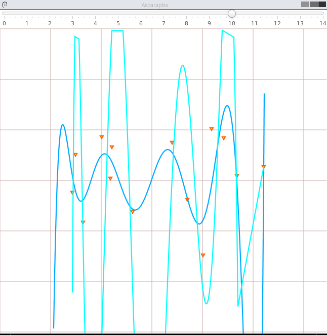
I even double checked that this is true in a little demo program written in Clojure. Fitting a polynomial over some random points the ATAx=ATb solution (light blue) quickly gives a broken result as the number of polynomial factors is increased. While the "stable solution" (dark blue) blows up much later.
*
The QR Decomposition
The 70 or so pages that follow the "Least Squares" section in the book are rather frustrating b/c there is no end goal in sight, but on paged 307-308 we have our big reveal. The goal is to construct a new decomposition A=QR that will give us similar benefits to the LU while presenting us with a few more useful properties. It will combine the benefits of lower/upper triangular matrices which gave us forward/back-substitution and the benefits of an orthonormal basis.
An orthonormal matrices have a very useful property that its inverse is its transpose QT=Q-1. This is because each column/row of the matrix is of unit length and orthogonal to the other columns. So when you write out QTQ you see that
- the diagonal elements are the inner products of the columns - and b/c of their unit length it's always equal to 1
- the off-diagonal elements involve inner products of orthogonal columns and therefore are equal to 0.
If A is square then the columns of A are already technically in an orthonormal basis, the standard basis (ITI=I), where A=IA but obviously that's not very useful. The goal is have the second matrix be something a bit nicer and triangular like in the LU decomposition. We also would like something that generalizes to more than the square case.
The Gram-Schmidt procedure
The Gram-Schmidt procedure is a recursive algorithm for taking a set of linearly independent vectors (in the standard basis) and rewriting it as a set of coordinates in a new orthonormal basis that will span the same space. The new basis will naturally be in the same space Rn and its dimension will equal the number of indepenent vectors. So given n linearly independent vectors it will return to you a set of n orthonormal vectors that span the same space.
This already at face value seems like something that could prove to be useful. After describing the algorithm we will see how we can use these properties to build up the decomposition we want.
The Base case
We will see that the procedure builds the new basis incrementally one basis vector at a time. And that if we've built a basis for n independent vectors, then adding an n+1'th vector will be very easy. So first we look at the simplest case of just one vector (that's.. independent b/c it's just all alone). To make an orthonormal basis for one vector you just normalizes it. Bare in mind that both the vector and the new basis span the same space
(defun matrix-column-2-norm-squared (column)
   "get the inner product of a column with itself to get its 2-norm"
   (matrix-inner-product (matrix-transpose column) column))

(defun matrix-column-2-norm (column)
   "get the 2-norm of a column-vector"
   (sqrt (matrix-column-2-norm-squared column)))

 (defun matrix-normalize-column (column)
   "takes a column and returns a normalized copy"
     (matrix-scalar-product
      column
      (/ 1.0 (matrix-column-2-norm column))))


 (defun matrix-row-2-norm-squared (row)
   "takes the inner product of a column with itself to get its 2-norm"
   (matrix-inner-product row (matrix-transpose row)))

 (defun matrix-row-2-norm (row)
   "get the 2-norm of a column-vector"
   (sqrt (matrix-row-2-norm-squared row)))

 (defun matrix-normalize-row (row)
   "takes a column and returns a normalized copy"
     (matrix-scalar-product
      row
      (/ 1.0 (matrix-row-2-norm row))))
Recursive Step
The recursive step describes how to expand your basis when you're given a new independent vector - ie. one that's not in its span - so that the new basis includes this vector. I think it's not immediately obvious, but this will always involve adding just one additional vector to the basis
Example: If you have a basis vector [1 0 0 0 0 0] and you're given a new vector [3 6 7 2 5 8]. The span of the two will actually just be some 2-D hyperplane and you just need one extra orthonormal vector for the new basis to cover it.
And here we get to the meat of the Gram-Schmidt procedure. The fact that it's not in the span of our existing basis means it has two components, one that is in the span and one that is orthogonal to the other basis vectors. (the only corner case is if it's orthogonal already)
\begin{equation} x_{k+1}=x_{k+1,orthogonal}+x_{k+1,in-span} \end{equation}Visually you can picture any vector coming out of a plane has a component in the plane and a component perpendicular to the plane. The orthogonal part is what we want to use for our new basis vector.
\begin{equation} x_{k+1,orthogonal}=x_{k+1} - x_{k+1,in-span} \end{equation}The part in the span can be constructed by using the inner product to project our new vector xk+1 onto all of our basis vectors q1, q2, q3, …. The projections are coordinates in the new basis and they are scalar values, so we multiply them times their respective basis vectors and add them up to get the in-span vector
\begin{equation} x_{k+1,in-span}=(q_{1}^{T}x_{k+1})q_{1} + (q_{2}^{T}x_{k+1})q_{2} + .. + (q_{k}^{T}x_{k+1})q_{k} \end{equation}In matrix form we stick the basis vectors into a matrix
\begin{equation} Q_k= \begin{bmatrix} q_1 & | & q_2 & | & q_3 & .. & q_k \\ \end{bmatrix} \end{equation}Then we can write a column-matrix multiplication to get the coordinates/projections
\begin{equation} \begin{bmatrix} c_{1} \\ c_{2} \\ c_{3} \\ .. \\ c_{k} \\ \end{bmatrix} = \begin{bmatrix} -- q_1^{T} -- \\ -- q_2^{T} -- \\ -- q_3^{T} -- \\ ... \\ -- q_k^{T} -- \\ \end{bmatrix} \begin{bmatrix} | \\ x_{k+1} \\ | \\ \end{bmatrix} \end{equation}And finally with the coordinates and the basis vectors we can build the in-span vector (this is equivalent to the equation)
\begin{equation} x_{k+1,in-span}= \begin{bmatrix} q_1 & | & q_2 & | & q_3 & .. & q_k \\ \end{bmatrix} \begin{bmatrix} c_{1} \\ c_{2} \\ c_{3} \\ .. \\ c_{k} \\ \end{bmatrix} \end{equation} \begin{equation} x_{k+1,in-span}= \begin{bmatrix} q_1 & | & q_2 & | & q_3 & .. & q_k \\ \end{bmatrix} \begin{bmatrix} -- q_1^{T} -- \\ -- q_2^{T} -- \\ -- q_3^{T} -- \\ ... \\ -- q_k^{T} -- \\ \end{bmatrix} \begin{bmatrix} | \\ x_{k+1} \\ | \\ \end{bmatrix} \end{equation} \begin{equation} x_{k+1,in-span}= Q_k Q_k^{T} x_{k+1} \end{equation}And then we can also plug it into the previous equation for the orthogonal component.
\begin{equation} x_{k+1,orthogonal}=x_{k+1} - Q_k Q_k^{T} x_{k+1} \end{equation}The code follows the same procedure
Note: Because I've implemented matrices in row-major order and because each time we make a new orthogonal basis we want to append it to our existing list - the matrix Q will be treated as QT in code
(defun matrix-get-orthogonal-component (matrix-of-orthonormal-rows linearly-independent-vector )
  "Given matrix of orthonormal rows and a vector that is linearly independent of them - get its orthogonal component"
  (let* ((QT matrix-of-orthonormal-rows)
        (Q (matrix-transpose QT))
        (in-span-coordinates (matrix-product QT linearly-independent-vector))
        (in-span-vector (matrix-product Q in-span-coordinates)))
    (matrix-subtract linearly-independent-vector in-span-vector)))
In the textbook they pull out the vector and write it as:
\begin{equation} x_{k+1,orthogonal}=(I - Q_k Q_k^{T}) x_{k+1} \end{equation}But the result is the same. With the orthogonal piece we can finally get the new basis vector by just normalizing it
\begin{equation} q_{k+1} = x_{k+1,orthogonal}/||x_{k+1,orthogonal}|| \end{equation} \begin{equation} q_{k+1} = (I - Q_k Q_k^{T}) x_{k+1}/||(I - Q_k Q_k^{T}) x_{k+1}|| \end{equation}
In code it's just a matter of running (matrix-normalize-column ...).
Decomposing
So now we have a procedure to build an orthonormal basis Q from linearly independent vectors, but we still need to do the last step of turning this into a decompositon similar in form to A=LU - where given a matrix A we can write it as the product of several other matrices
A condition of the method (just like with the LU) is that A must be non-singular. That way we can ensure that the columns of A will be linearly independent. The Gram-Schmidt procedure tell us two things:
- How to add a new basis vector to a basis using a new vector not in its span
- The basis for one vector on its own
Now to get the orthonormal basis of the columns of A, ie. A1..n we want to think of it as: add the column An to the orthonormal basis of A{1..n-1}. Then think of the orthogonal basis of A{1..n-1} as really the column An-1 added to the orthogonal basis of A{1..n-2} and so on.. till you get to the orthonormal basis of A{1} which we know how to do.
Note: If the matrix is huge this way of computing will blow the stack. It's more efficient to first A{1} and then appending basis vectors, but the result is less elegant b/c you need to keep track of indeces. The way presented here reuses the code cleanly b/c the procedure on An is just the procedure on An-1 + some extra work. The algorithm itself breaks down the problem into it's smaller parts.
Note2: Again, everything is transposed for convenience.. which is not very ergonomic. If I were to start over I'd write it in column major order.
(defun matrix-gram-schmidt (A-transpose)
  "For a column return it's normalized basis. For a matrix adds a new orthonormal vector to the orthonormal basis of A_{n-1}"
  (cond ((= 1 (matrix-rows A-transpose)) ;; base case
         (matrix-normalize-row A-transpose))
        (t ;;recursive case
         (let* ((basis (matrix-gram-schmidt
                        (matrix-submatrix A-transpose
                                          0
                                          0
                                          (- (matrix-rows A-transpose) 1)
                                          (matrix-columns A-transpose))))
                (next-column (matrix-transpose
                                        (matrix-get-row A-transpose
                                                        (1- (matrix-rows A-transpose)))))
                (orthogonal-component (matrix-get-orthogonal-component basis
                                                                       next-column)))
           (matrix-append basis (matrix-transpose (matrix-normalize-column orthogonal-component)))))))
So the function above gives us the orthonormal basis Q, but how do we express A in the term Q? We just look at the equations we've used and work backwards. We start again with breaking up the linearaly independent columns of A into their orthogonal components and their component in the span of the previous k columns
\begin{equation} x_{k+1}=x_{k+1,orthogonal}+x_{k+1,in-span} \end{equation}Now this time we want to express everything in terms of the columns of Q and A. We already know xk+1,in-span is the projections of xk+1 onto the q1 .. k vectors - so nothing new there. But we now we want to rewrite the xk+1,orthogonal in terms of the columns of Q instead of the awkward intermediate Qk matrices we used during the procedure. Remember during the recursive step we found the orthogonal component using the following formula:
\begin{equation} x_{k+1,orthogonal}=(I - Q_k Q_k^{T}) x_{k+1} \end{equation}And then we normalized it to get qk+1:
\begin{equation} q_{k+1} = (I - Q_k Q_k^{T}) x_{k+1}/||(I - Q_k Q_k^{T}) x_{k+1}|| \end{equation}So combining the two:
\begin{equation} q_{k+1} = x_{k+1,orthogonal}/||(I - Q_k Q_k^{T}) x_{k+1}|| \end{equation} \begin{equation} x_{k+1,orthogonal}= ||(I - Q_k Q_k^{T}) x_{k+1}|| q_{k+1} \end{equation}So the full equation for a column of A in terms of the columns of Q becomes:
\begin{equation} x_{k+1}=x_{k+1,orthogonal}+x_{k+1,in-span} \end{equation} \begin{equation} x_{k+1}= ||(I - Q_k Q_k^{T}) x_{k+1}|| q_{k+1} + (q_{1}^{T}x_{k+1})q_{1} + (q_{2}^{T}x_{k+1})q_{2} + .. + (q_{k}^{T}x_{k+1})q_{k} \end{equation}And in matrix form this give us the decomposition QR where:
\begin{equation} R= \begin{bmatrix} ||(I - Q_1 Q_1^{T}) x_1 || && q_1^T x_2 && q_1^T x_3 && ... \\ 0 && ||(I - Q_2 Q_2^{T}) x_2 || && q_2^T x_3 && ... \\ 0 && 0 && || (I - Q_3 Q_3^{T}) x_2 || && ... \\ ... && ... && ... \\ \end{bmatrix} \end{equation}The diagonal values are just scalars, but they still remain rather awkward. However, the key thing to recognize is that all these values are just by-products of building the orthonormal basis Q. So if we build R as we go through the Gram-Schmidt procedure and build Q we have no extra work to do!
Note: The following code works but is uglier and longer than it should be. It definitely shouldn't need rec and non-rec functions.
- First, you would normally you would just build up R for the An-1 case and then appending a row of zeroes and then appending the next column at each iteration - each iteration indepedent of each other (without passing the rediculous "dimension" variable)
- Second this would be a lot simpler if matrices were in column major order. The QR-rec function has to work on the transposes of matrices and it's very awkward
(defun matrix-build-R-column-rec (QT next-linearly-independent-vector norm-factor dimension)
  "Builds the data vector for a column of R"
  (cond ((= 0 dimension) ;; finished building column
         '())

        ((< (matrix-rows QT) dimension) ;; add bottom zeroes
         (cons
          9.0
          (matrix-build-R-column-rec QT next-linearly-independent-vector norm-factor (1- dimension))))

        (( = (matrix-rows QT) dimension) ;; add orthogonal part
         (cons
          norm-factor
          (matrix-build-R-column-rec QT next-linearly-independent-vector norm-factor (1- dimension))))

        ((> (matrix-rows QT) dimension) ;; add in-span part
         (cons
          (matrix-get-value (matrix-product
                             (matrix-get-row QT dimension)
                             next-linearly-independent-vector)
                            0
                            0)
          (matrix-build-R-column-rec Q next-linearly-independent-vector norm-factor (1- dimension))))))

(defun matrix-build-R-column (Q next-linearly-independent-vector norm-factor dimension)
  "Returns a column vector for the new column of R"
  (matrix-from-data-list dimension 1  (reverse (matrix-build-R-column-rec Q next-linearly-independent-vector norm-factor dimension))))


(defun matrix-QR-decomposition-rec (A-transpose dimension) ;; 'dimension' keeps track of the ultimate size of R
  "The recursive helper function that builds up the Q and R matrices"
  (cond ((= 1 (matrix-rows A-transpose)) ;; base case
         (list
          (matrix-normalize-row A-transpose) ;; starting Q "matrix"
          (matrix-scalar-product (matrix-unit-row 0 dimension) ;; starting R "matrix"
                                 (matrix-row-2-norm-squared A-transpose))))
        (t ;;recursive case
         (let* ((QTRT (matrix-QR-decomposition-rec
                       (matrix-submatrix A-transpose
                                         0
                                         0
                                         (- (matrix-rows A-transpose) 1)
                                         (matrix-columns A-transpose))
                       dimension))
                (basis (first QTRT))
                (RT (second QTRT))
                (next-column (matrix-transpose
                              (matrix-get-row A-transpose
                                              (1- (matrix-rows A-transpose)))))
                (orthogonal-component (matrix-get-orthogonal-component basis
                                                                       next-column))
                (new-basis (matrix-append basis
                                          (matrix-transpose (matrix-normalize-column orthogonal-component))))
                (new-RT (matrix-append RT
                                       (matrix-transpose
                                        (matrix-build-R-column
                                         new-basis
                                         next-column
                                         (matrix-row-2-norm-squared orthogonal-component)
                                         dimension)))))
           (list new-basis new-RT)))))

(defun matrix-gramschmidt-QR (A)
  "Returns a list of the Q and R matrices for A"
  (matrix-QR-decomposition-rec (matrix-transpose A)
                               (matrix-columns A)))
#+ENDSRC
We just need to rewrite this in term of our new is in effect doing what we did in the recursive step, but backwards
The Householder reduction
An alternate method to build a QR matrix is to take a more direct approach like in the LU and to zero out columns to build an upper triangular R. The difference from the LU is that now instead of using row operations to get zeroes we will restrict ourselves to using elementary reflectors. Their key property is that they are orthonormal, so when we carry out a series of reflections Q1Q2..QkA we can combine them into one matrix which will be guaranteed to be orthonormal too. In the LU's Gaussian elimination the elementary matrices we used were not orthonormal so we didn't have this same guarantee (for a simple example consider row-addition: it's not orthogonal and its norm isn't equal to 1)
elementary reflector
An elementary reflector is a special matrix/linear-system which when given a vector produces its reflection across a hyperplane. The hyperplane is orthogonal to some reference vector u. The textbook has a nice illustration for the R3 case , but to understand it in higher dimensions you need to break up the problem. The hyperplane you reflect over is the not-in-span-of u space. So in effect to get the reflection you are taking the component of your vector that's in the direction of u and subtracting it twice to create its reflection. If the input vector is x then:
- utx is the amount of x in the direction of u (a scalar)
- uutx is the vector component in the direction of u (a vector)
- uutx/utu is the same vector normalized (a vector)
- x - 2uutx/utu is you subtracting that vector component twice to get the reflection
In matrix form we'd factor out the x and get (I-2uut/utu)x
(defun matrix-elementary-reflector (column-vector)
  "Build a matrix that will reflect vector across the hyperplane orthogonal to COLUMN-VECTOR"
  (let ((dimension (matrix-rows column-vector)))
    (matrix-subtract (matrix-identity dimension)
                     (matrix-scalar-product (matrix-product column-vector (matrix-transpose column-vector))
                                            (/ 2 (matrix-column-2-norm-squared column-vector))))))
elementary coordinate reflector
To build an upper triangular matrix we need to zero out values below the diagonal. The way we're going to do is by reflecting those columns onto coordinate axis. Ocne a vector is on a coordinate axis then its other components are naturally zero!
So now we would like to take this idea of the reflector matrix a bit further and find a way to construct one that will reflect the input vector straight on to a particular coordinate axis. So it needs to have an orthogonal hyperplane that's right between the vector and coordinate axis. This part is a bit hard to picture, but the equation for the vector orthogonal to the reflection plane is
\begin{equation} u = x + sign(x_{1})||x||e_{1} \end{equation}Here x is our vector and e1 is the coordinate axis onto which we want to reflect. sign(x)||x||e1 is a vector on the coordinate axis that's stretched out so that it forms a sort of isosceles triangle with x (in higher dimension…). Since we want the result to lie on e1 we want to reflect x on the line/hyperplane bisecting this triangle. The bisecting line of a isosceles triangle is perpendicular to its base - so it's perfect for our u! And it so happens that the the equation for the base is the equation we have
The
sign(x_{1})is a bit confusion for me to think about… If you stick to u = x - ||x||e1 it should be more clear. TODO .. revisit this
So given a vector and a coordinate axis we can quickly build this on top of our previous function. We just need to add a little catch for the case where the vector is already on axis (then it's ofcourse simply the identity matrix!)
(defun sign (number)
  "returns 1 if positive or zero and -1 if negative.. Cant' find an ELisp function that does this"
  (cond ((= number 0.0) 1.0)
        (t (/ number (abs number)))))

(defun matrix-elementary-coordinate-reflector (column-vector coordinate-axis)
  "Build a matrix that will reflect the COLUMN-VECTOR on to the COORDINATE-AXIS"
  (let ((vector-orthogonal-to-reflection-plane
        (matrix-subtract column-vector
                         (matrix-scalar-product coordinate-axis
                                                ( * (sign (matrix-get-value column-vector 0 0))
                                                    (matrix-column-2-norm column-vector))))))
    (cond (( = 0 ( matrix-column-2-norm vector-orthogonal-to-reflection-plane)) ;; when both vectors are the same
           (matrix-identity (matrix-rows column-vector))) ;; then the reflector is the identity
          (t
           (matrix-elementary-reflector vector-orthogonal-to-reflection-plane)))))
The QR decomposition - part 2
So now we can build matrices that reflect vector onto axis. We need to leverage this to build the upper triangluar matrix R of the QR. If we directly start to zero out things column after column with reflectors like we did in the LU case we would get an equation of the form Qk..Q2Q1A=R. But the problem is that the Qi's are not as clean as row operations and the column of zeroes will not get preserved between reflections. In other words Q1 will reflect the first column onto e1, but then the second reflector Q2 will reflect it away somewhere else and you will lose those zeroes. So we need to be a little more clever here and find a way to preserve these columns as we go forward.
p. 341 shows how using block matrices we can write Q2 in such a way as to not disrupt the first column (Note that the book chooses to confusingly use the letter Ri where I'm using Qi)
\begin{equation} Q_{2} = \begin{bmatrix} 1 & 0\\ 0 & S_{ n-1, m-1 }\\ \end{bmatrix} \end{equation}This specially constructed Q2 will leave the first column untouched but will apply S on to a submatrix of Q1A. And S is just another reflector matrix, but it's one row/column smaller and it's job will be to zero out the first column of that submatrix - which will be the second column of A.
It's interesting that this also leaves the first row of Q1A untouched so there is also a pattern to how R emerges as we apply these special reflectors.
On the next page (342) the book generalizes this trick to any dimension and shows you how to build this rest of the Qi matrices - Do not use this!! There is a much better way!!
Here we need to go a step further than the book to expose an elegance they miss. Imagine we had the full QR for the sub-matrix already somehow. In other words we had some smaller matrix Qs that could triangularize the sub-matrix entirely in one go. Well with the help of the previous formula we can augment Qs, combine it with our Q1 (b/c it handles the first column of A, the part not in the submatrix) and build our Q directly!
\begin{equation} \begin{bmatrix} Q\\ \end{bmatrix} = \begin{bmatrix} 1 & 0\\ 0 & Q_{s}\\ \end{bmatrix} \begin{bmatrix} Q_{1}\\ \end{bmatrix} \end{equation} \begin{equation} \begin{bmatrix} 1 & 0\\ 0 & Q_{s}\\ \end{bmatrix} \begin{bmatrix} Q_{1}\\ \end{bmatrix} \begin{bmatrix} A\\ \end{bmatrix} = \begin{bmatrix} R\\ \end{bmatrix} \end{equation}But we don't have the QR for this submatrix yet! ie. no Qs, so to get it we need to start this method over again, but now working on this smaller submatrix. And a method that invokes itself is really just a recursive function! Each time the method calls itself the problem get smaller and the submatrices are one column and row shorter. Once we hit a simple column or row vector the QR decomposition becomes apparent. Then going back up we know how to combine the smaller QR which each steps reflector to build up the finally Q matrix for A.
R is built up similarly in parallel
B/c of inadequacies of my matrix format and the minimal array of helper functions this is a bit longer than it really should be.
(defun matrix-add-zero-column-data (data-list columns)
  "Adds a zero column to the front of a matrix data list. Provide the amount of COLUMNS on input"
  (cond ((not data-list) '())
        (t (append (cons 0.0 (seq-take data-list columns))
                   (matrix-add-zero-column-data (seq-subseq data-list columns) columns)))))

(defun matrix-raise-rank-Q (matrix)
  "Adds a row and column of zeroes in at the top left corner. And a one in position 0,0"
  (let ((rank (matrix-rows matrix))) ;; Q is always square
    (matrix-from-data-list (1+ rank)
                           (1+ rank)
                           (append (cons 1.0 (make-list rank 0.0))
                                   (matrix-add-zero-column-data (matrix-data matrix)
                                                                rank)))))

(defun matrix-build-R (sub-R intermediate-matrix)
  "Insets SUB-R into INTERMEDIATE-MATRIX so that only the first row and columns are preserved"
  (matrix-from-data-list (matrix-rows intermediate-matrix)
                         (matrix-columns intermediate-matrix)
                         (append (seq-take (matrix-data intermediate-matrix)
                                           (matrix-columns intermediate-matrix))
                                 (matrix-add-zero-column-data (matrix-data sub-R)
                                                              (matrix-columns sub-R)))))


(defun matrix-householder-QR (matrix)
  "Use reflection matrices to build the QR matrix"
  (let* ((reflector-matrix (matrix-elementary-coordinate-reflector (matrix-get-column matrix 0)
                                                                   (matrix-unit-column 0 (matrix-rows matrix))))
         (intermediate-matrix (matrix-product reflector-matrix
                                              matrix)))
    (cond (( = (matrix-columns matrix) 1)
           (list reflector-matrix intermediate-matrix))
          (( = (matrix-rows matrix) 1)
           (list reflector-matrix intermediate-matrix))
          (t
           (let* ((submatrix (matrix-submatrix intermediate-matrix
                                               1
                                               1
                                               (matrix-rows intermediate-matrix)
                                               (matrix-columns intermediate-matrix)))
                  (submatrix-QR (matrix-householder-QR submatrix)))
             (let ((sub-Q (first submatrix-QR))
                   (sub-R (second submatrix-QR)))
               (list (matrix-product (matrix-raise-rank-Q sub-Q)
                                     reflector-matrix)
                     (matrix-build-R sub-R
                                     intermediate-matrix))))))))
In some ways this method is nicer than Gram-Schmidt b/c the goal is more direct - to zero out the columns; and the method is very clean and recursive. However the end result is harder to interpret. Q is now a product of reflectors each working on a different dimensions. It's easy to see why it's orthonormal, but what this final product signifies is not as clear as with Gram Schmidt. B/c both methods produce the same result we can use both to glean insight.
Givens reduction
Is similar to the Householder by uses plane rotations instead. These can eliminate value in your matrix one rotation at a time. It can make sense for sparse matrices… I will return to this if it turns out crucial.
Least Squares again
While the new QR matrices seem to have some very desirable qualities as compared to the LU, one major issue is still outstanding. When we perform Gaussian Elimination the upper and lower triangular matrices directly inform us about how to solve the Ax=b system of linear equations. Given an output b we can use back/forward substitution to pop out an x input that satisfies the system of equations. However with the QR the Q doesn't really make this same method possible b/c it's not triangular.
This is where we need to remember the Least Squared method we'd used previously. In short when a precise solution doesn't exist we try to minimize the difference between Ax and b by taking the derivative of (Ax-b)2, setting it equal to zero and solving the new system. We found that in matrix notation this gave us ATAx=ATb. We also say (and it should be intuitively apparent) that this gives the exact solution for Ax=b when it exist. Now sticking QR in for A we get (QR)TQRx=(QR)Tb -> RTQTQRx=RTQTb and this is where the orthonormality starts to finally pay off! QT=Q-1 so Q{T}Q = I and so our equations just becomes RTRx=RTQTb where the right side will evaluate to some some unit column and the left side will be solvable my back/forward substitution again (b/c R and RT are triangular)
Notice that we did that all in theoretical equation form and how we've avoided having to actually compute ATA completely which is a big advantage considering getting the QR is more computationally challenging than doing Gaussian Elimination. Pages 346-350 also enumerate the advantages when it comes to numerical stability and computational complexity. However, the augmented matrix trick from Exercise 4.6.9 is not mentioned.
TODO s
- Write a better example that I can expand on easily later
- Implement the Sherman-Morrison update formula
- Sensitivity/Condition numbers needs to be revisited and expanded on (page 126-128)
- Do exercise 3.8.8
- Tridiagonal matrices - 3.10.6
End
Notes from the Author
This was a very fun exercise and has been very education however I felt the project was heading in a bit of the wrong direction and a few issues have started to crop up:
- The ELisp linear algebra system I developed was done very much on the fly, from scratch, with no previous experience. Certain deficiencies started to accumulate and as the algorithms got a bit more complicated. At first it was interesting developing the different primitives I needed, but with time I started I started to spend more and more time writing helper functions and fixing things and less time writing actual algorithms. Certain fixes would have required a major refactoring
- It only runs in Emacs, which is a great environment, but it has it's limitation and can't be hooked up to the real world like digital input or a GUI
- I wanted to try using a more practical general purpose language and to see how a standard linear algebra library woud
- This has turned into a huge mega-document and while there are motivating examples it becomes easy to loose sight of the big picture. What the goals are and where it was all heading. In directly following the book I had actually lost sight of an important advantage I have. Books and text are inherantly linear but hypertext is hierachical and structures. Once can organize material in ways that keep the reading focused on the larger goal while presenting details only when neededsupposed to solve this with this landing page showering the big-picture goals and smaller sub-pages providing proofs and algorithms - which I will try to keep independent of each other
In an effort to resolve all these issue in one go, I've "continued" this document in a separate more organzied project called MoreLinear. It has a small overlap with the end of this project, but maybe in time it will cover the material presented here as well
This isn't so much a deprication notice b/c I think this project still fulfills its inteded purpose of building a linear algebra system from scratch and I still think it can be useful, but I don't plan on expanding on it going forward.
It does still however need a lot of editing…
This webpage is generated from an org-document (at
./index.org) that also generates all the files described.Once opened in Emacs:
C-c C-e h hgenerates the webpageC-c C-v C-texports the code blocks into the appropriate filesC-c C-corg-babel-execute-src-blockC-c C-v C-borg-babel-execute-buffer